Data Base
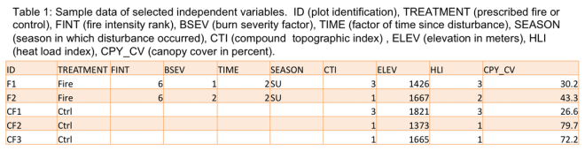
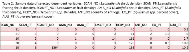
A desired outcome of this research is to highlight the influences that eight different predictor variables (based on terrain, fire, and forest factors) have on 16 different bear foods (total of 21 response variables) across two control variables (prescribed fires and adjacent forested controls). A simplified version of the data is outlined in table 1 and table 2. The sampling units, control variables, and predictor variables are illustrated in table 1, while a representative sample of the response variables are illustrated in table 2. In table 1, the "ID" column represents the different plot locations (sampling units). The control variables are represented by either the "Fire" for prescribed fire or "Ctrl" for control in the "TREATMENT" column. Fire based predictor variables are represented by "FINT" (fire intensity), "BSEV" (burn severity), "TIME" (time since fire) and "SEASON" (season of ignition). Since these are fire based variables they are not applicable to the controls. Terrain based predictor variables are represented by "CTI" (compound topographic index), "ELEV" (elevation of the site in meters) and "HLI" (heat load index). Forest canopy cover (%) was the only forest based predictor variable used in this experiment and when also can be modeled as response variable to the other predictor variables.
A desired outcome of this research is to highlight the influences that eight different predictor variables (based on terrain, fire, and forest factors) have on 16 different bear foods (total of 21 response variables) across two control variables (prescribed fires and adjacent forested controls). A simplified version of the data is outlined in table 1 and table 2. The sampling units, control variables, and predictor variables are illustrated in table 1, while a representative sample of the response variables are illustrated in table 2. In table 1, the "ID" column represents the different plot locations (sampling units). The control variables are represented by either the "Fire" for prescribed fire or "Ctrl" for control in the "TREATMENT" column. Fire based predictor variables are represented by "FINT" (fire intensity), "BSEV" (burn severity), "TIME" (time since fire) and "SEASON" (season of ignition). Since these are fire based variables they are not applicable to the controls. Terrain based predictor variables are represented by "CTI" (compound topographic index), "ELEV" (elevation of the site in meters) and "HLI" (heat load index). Forest canopy cover (%) was the only forest based predictor variable used in this experiment and when also can be modeled as response variable to the other predictor variables.
Data Exploration
Normality
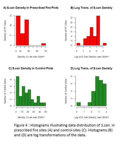
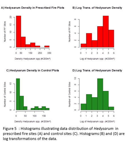
Many of the response variables (grizzly bear foods) at the majority of the sampling locations were entirely absent or extremely low in density. These absences, or zero values, generated data distributions that have positive skews and as a result caused non-normal distribution. Even the more abundant grizzly bear foods such as S.canadiensis (Fig. 4) and Hedysarum spp. (Fig. 5) indicate a a significant positive skew in both prescribed fires and controls as indicated by the histograms. A square root transformation and a log transformation (Fig. 4 and 5) method were approached to reduce the effect of the inflated zero values as well as outliers (Fig. 6). These transformations reduced the positive skew however, according to the Shipiro-Wilk test, not enough to redeem the distributions as "normal." Figure 4 and 5 illustrate the histograms of S.canadiensis and Hedysarum spp. plant density distributions and the effect of a log transformation on these. With none of the dependant variables following a normal distribution, a non-parametric analysis of the raw data values was selected.
Normality
Many of the response variables (grizzly bear foods) at the majority of the sampling locations were entirely absent or extremely low in density. These absences, or zero values, generated data distributions that have positive skews and as a result caused non-normal distribution. Even the more abundant grizzly bear foods such as S.canadiensis (Fig. 4) and Hedysarum spp. (Fig. 5) indicate a a significant positive skew in both prescribed fires and controls as indicated by the histograms. A square root transformation and a log transformation (Fig. 4 and 5) method were approached to reduce the effect of the inflated zero values as well as outliers (Fig. 6). These transformations reduced the positive skew however, according to the Shipiro-Wilk test, not enough to redeem the distributions as "normal." Figure 4 and 5 illustrate the histograms of S.canadiensis and Hedysarum spp. plant density distributions and the effect of a log transformation on these. With none of the dependant variables following a normal distribution, a non-parametric analysis of the raw data values was selected.
|
|
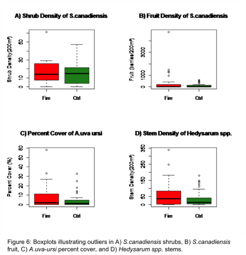
Outliers
An observation of the boxplots for the different variables (Fig. 6), indicates a significant amount of outliers. These outliers represent greater abundances of grizzly bear foods at these sampling locations. These high abundances reveal important data and therefor could not be omitted from the analysis. These outliers contributed to the difficulty of establishing a normal distribution with transformations. They also create significantly increase the variance of the data.
Homogeneity of Variance
Residuals of each model were plotted against the fitted values to compare the amount of variability in the samples. The residual vs. fitted value graphs revealed that there was substantial heterogeniety of variance for many of the variables. This was confirmed using a Bartlett test.
Independence
To ensure that the observations were independent to one another each site was randomly selected through GIS. As well, each site was a minimum of 1500m distance apart to avoid the effects of pseaudoreplication.
